Last time I participated in the Practice round of Google Code Jam 2018. It was a fun experience, so on 2018-04-07 I went for the Qualification round.

While practice round took about 7 hours to complete, the qualification round topped that requiring about 10h of work. As previously, there 4 problems with one visible and one hidden result each. I managed to correctly complete 1/2 tests for the first three, and then 2/2 tests for the fourth one for a total of 55/100 points. Bummer!

But, here’s how I approached the problems.

1. Saving the universe again

Problem description.

In short, a killer robot is executing a program, which consists of 2 instructions. C charges the weapon, doubling the damage, S shoots the weapon. Hero can swap two adjacent instructions, but want to do so as few times as possible. What is the minimum number of such changes have to be made so that the robot doesn’t do more than a specific amount of damage? E.g. SCSS: shoot for 1 damage, charge damage to two, shoot for 2 damage (total=1+2=3), shoot for 2 damage (total=1+2+2=5).

By Swfung8 - Own work, CC BY-SA 3.0

To start with, having to swap instructions around sounds similar to Bubble Sort, where you swap around adjacent elements if left one is bigger than the right one. Here idea is similar as well.

The second point we can notice is that CHARGE instruction doubles damage for any future SHOOT instructions, but does not do any damage by itself. So a) any CHARGE instruction after the last SHOOT instruction is irrelevant and can be discarded from the search, and b) we can move CHARGE instructions to the right.

There is a special case to account for: when is it impossible to stay under a specific amount of damage? And the limit is that if all SHOOT instructions are on the left hand side (and are worth 1 point each), if that exceeds the damage limit - there’s nothing else we can do to avoid that damage. So the first step is to check if it’s even possible to achieve the intended damage target:

def count_instructions(instruction, instructions):
    return instructions.count(instruction)

def solve(max_damage, instructions):
    if count_instructions(SHOOT, instructions) > max_damage:
        return 'IMPOSSIBLE'
    # ...

As for the core behavior, which instructions would affect the end result the most? Well, CHARGE instructions stack, so if you had 5 CHARGE instructions and then a SHOOT instruction - that’s 2 ^ 5 = 32 damage points. But, if we swap the last CHARGE instruction with SHOOT instruction - that cuts damage in half (2 ^ 4 = 16).

So the main algorithm is as follows:

1. Trim any trailing CHARGE instruction, that don’t have a SHOOT instruction after them. We’ve already established it - they don’t affect the end result;
2. Find the rightmost CHARGE instruction that has a SHOOT instruction following it, and swap the two. Doing so will reduce the power of that SHOOT instruction by 50% - the most we can achieve at that point;
3. Repeat until the estimated damage is low enough.

def prune_instructions(instructions):
    last_instruction = instructions[-1]
    while instructions != [] and last_instruction != SHOOT:
        instructions.pop()
        last_instruction = instructions[-1]
    return instructions

def swap_with_left(index, instructions):
    start_len = len(instructions)
    instructions[index-1:index+1] = [instructions[index], instructions[index-1]]
    return instructions

def swap_last_shoot_with_charge(instructions):
    instructions.reverse()
    first_charge = instructions.index(CHARGE)
    instructions = swap_with_left(first_charge, instructions)
    instructions.reverse()
    return instructions

def solve(max_damage, instructions):
    if count_instructions(SHOOT, instructions) > max_damage:
        return 'IMPOSSIBLE'
    max_changes = 100
    changes = 0

    while count_damage(instructions) > max_damage and changes < max_changes:
        instructions = prune_instructions(instructions)
        instructions = swap_last_shoot_with_charge(instructions)
        changes += 1

    return changes

And that’s it. However, this passed only 1 out of 2 tests.

Looking at it again, it may be due to me limiting max_changes to 100 - I forgot to consider that number of instructions can be as high as 30. Meaning that if four rightmost instructions are SHOOT - the algorithm would prematurely terminate, yielding a wrong answer. Gah! It should’ve been a bit higher, maybe 10e3 or 10e4.

2. Trouble sort

Problem description.

A sorting algorithm is given in pseudocode, and it’s not functioning correctly. Our job is to write a program that would check its results, writing OK if it worked normally, or outputting the index of an element preceeding a smaller number.

Sounds simple enough. We could memorize the first element of the sorted list, loop through the sorted list, making sure that the current element is not smaller than the previous one. If there is a failure - we found the problem with the previous element. If it passed - we return OK.

# Given in problem description
def trouble_sort(L):
    done = False
    while not done:
        done = True
        for i in range(len(L)-2):
            if L[i] > L[i+2]:
                done = False
                temp = L[i:i+2+1]
                temp.reverse()
                L[i:i+2+1] = temp

    return L

def solve(N, values):
    L = trouble_sort(values)

    last_value = L[0]
    for (i, x) in list(enumerate(L))[1:]:
        if last_value > x:
            return i-1
        last_value = x

    return 'OK'

This passed the first visible test, but failed the second hidden test, exceeding the time limit. What I forgot to take into account is the “special note”:

Notice that test set 2 for this problem has a large amount of input (10^5 elements), so using a non-buffered reader might lead to slower input reading. In addition, keep in mind that certain languages have a small input buffer size by default.

So the solution exceeded the 20 second time limit. Not sure yet if input is really the full problem, e.g. generating the full enumerated list is not ideal, it would’ve been smarter to leave the generator as is, computing values lazily. But still, that’s another blunder.

3. Go, Gopher!

Problem description.

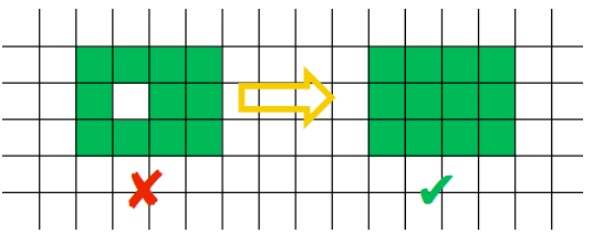
In short, we are given a number of cells that need to be marked. But, the way these cells have to be oriented in a grid has to form a continuous rectangle with no gaps. E.g. for input of A=20 one might choose a grid of 4x5 rectangle. The tricky part is how cells can be marked. The program has to specify which cell it wants to mark, but the testing program can mark that or any one of its 8 neighboring cells randomly, telling you which cell has been actually marked. And even if a cell has already been marked - the Gopher may mark it multiple times. Doing so doesn’t do anything extra, only wastes the guess.

I don’t know how to deal with randomness in such a case. Perhaps one could try gaming the pseudorandom number generator, but it’s unlikely.

A perhaps more likely approach could be to start with a couple arbitrary guesses, compute probabilities for available cells find the next best guess that way, and try to evolve the grid to fit into desirable shape with a specific area. But such approach sounds complex, so instead I went for the (very) naive approach.

The RNG guesses uniformly, so probability that each of the 3x3 cells gets prepared is 1/9. So we could orient the 3x3 block in such a way that it always fits within the area we want to fully mark, and move the block from side to side, up and down, keeping guessing until we’re lucky and we fill the intended grid, or we run out of guesses. On the first visible test where N=20 it’s pretty likely that we’ll fill up a 4x5 grid, but I’m not so confident about the N=200 and 14x15 grid.

Something to keep in mind is how much of an overlap there is between two adjacent block guesses. The larger the overlap - the more likely overlapped cells will get marked, but the fewer guesses there are to cover the rest of the board. And edges and especially corners are a problem for such approach, as e.g. for a corner to be filled in there will only be as many opportunities as times one can cover the full board.

I first tried moving one column and one row at a time, and that was enough to pass the interactive local test and the visible test. But I was worried about corners and edges of the rectangle for the N=200 case, so instead I opted moving two columns and two rows at a time, reducing overlap between 2 adjacent guess blocks from 2 cells to 1 cell, but increasing the number of times the full board can be covered by about a factor of 2.

MAX_TRIES = 1000
HALT = 'HALT'

def has_test_failed(coords):
    return coords == [-1, -1]

def has_test_succeeded(coords):
    return coords == [0, 0]

def mark_filled_cell(cell, board):
    board[tuple(cell)] = True
    return board

def coords_offset(center, offset_x, offset_y):
    return (center[0]+offset_x, center[1]+offset_y)

def get_cell(coords, board):
    return tuple(coords) in board

def mask(center, board):
    """ List of cells in a guess block with a given center cell """
    result = []
    for i in range(3):
        for j in range(3):
            result.append(get_cell(coords_offset(center, i-1, j-1), board))
    return result

def solve(A):
    width = math.floor(math.sqrt(A))
    height = math.ceil(math.sqrt(A))
    WINDOW = 3
    board = {}
    guess = 0

    while guess < MAX_TRIES:
        # Leave out edges
        w = list(range(width))[1:-1]
        if width % 2 == 0: w.append(width - 1)
        h = list(range(height))[1:-1]
        if height % 2 == 0: h.append(height - 1)

        for i in w:
            for j in h:
                center = (i+1, j+1)
                if all(mask(center, board)):
                    # Given block is fully filled up
                    continue

                write_answer(center)
                filled_cell = read_ints()
                if has_test_failed(filled_cell):
                    return HALT
                if has_test_succeeded(filled_cell):
                    return
                board = mark_filled_cell(center, board)
                guess += 1
    return HALT

This passed 1 out of 2 tests, failing with a “Wrong answer” on the “N=200” hidden test. I didn’t expect the second one to pass - it was unlikely to do so. But, as a third option I would have tried placing guess blocks without any overlap at all, increasing the number of full rectangle guess coverage even further, in the hopes of hitting the right chance.

4. Cubic UFO

Problem description.

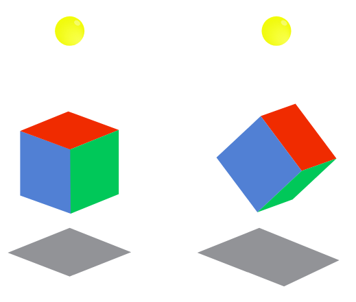
In short, there is a 3D cube hanging above ground and casting a shadow. How should we rotate the cube to get its shadow’s area to be as close as possible to a specific number? For simplicity’s sake, the cube’s center point is at origin (0, 0, 0), cube is 1km wide, and its shadow is being cast onto a screen 3km under the origin.

It was actually fairly straightforward, but tough to implement, requiring knowledge of multiple algorithms and implementation of matrix operations. I think I’ve spent most of my time on this problem.

The first idea was that maybe there is a mathematical formula describing an area of any cube slice through its center point. A quick search hasn’t yielded much, so this idea was abandoned.

Instead the requirements of the problem suggested a different approach. Notice that precision of answers has to be within about 10e-6, and inputs for all test cases are very precise, e.g. (1.000000, 1.414213, 1.732050). This raised an idea from numerical methods class - maybe if we could rotate the cube slightly, we could discover directions in which rotation gave the closest shadow area, and following those directions would get closer and closer to the desired answer.

From numerical methods class I vaguely remembered Newton’s method and from neural networks class came Gradient Descent.

On the right path, allowing to get closer and closer to the solution, but it’s only part of the solution. Full implementation still requires knowing how to calculate verteces and faces of the rotated cube, project those points onto 2D space, and calculate the area of cube’s shadow.

4.1. Cube rotations

First we need a way to describe the relevant coordinates. What would be the coordinates of each of the verteces and faces?

Well, cube’s center point is at origin, and the cube itself is 1km wide. That would mean its faces are 1km/2 = 0.5km away from the center point. So such points can be described as vectors, e.g. (0.5, 0, 0), (0, 0.5, 0), (0, 0, 0.5) vectors would give center points for three of the faces of the cube, and similarly replacing 0.5 with -0.5 would give the other 3 faces.

Likewise, cube’s verteces can be described as 3D vectors as well, e.g.: (0.5, 0.5, 0.5), (0.5, 0.5, -0.5), …, (-0.5, -0.5, -0.5).

So we have 2 sets of vectors, one to describe the 3 relevant face center points, and the other one for cube’s 8 verteces.

It’s been a while since my last linear algebra class, but after some searching I found that there are such things as Rotation matrices. Multiplying a vector by the appropriate rotation matrix would return the rotated vector. I would encourage you to read the full wiki article.

But doing so would require implementing some basic matrix functionality. Interestingly, as I was looking for solutions to this problem, many StackOverflow commentators suggested solutions using Numpy or Scikit, however such libraries are not available in Code Jam.

I’ve implemented matrices as follows. Matrix notation was [(a11, a21, ..., an1), (a12, ..., an2), ... (a1m, ..., anm)], where i denotes the row, and j denotes the column for a n row and m column (nxm) matrix. So the tuple in this case meant a column vector. Visually somewhat comfusing as they are written out in columns.

def matrix_column(A, column):
    return list(A[column])

def matrix_row(A, row):
    return list(map(lambda v: v[row], A))

def multiply_matrix(A, B):
    n = len(A[0])
    m = len(A)
    p = len(B)

    result = []
    for j in range(p):
        acc = []
        for i in range(n):
            c = 0
            for (a, b) in zip(matrix_row(A, i), matrix_column(B, j)):
                c += a * b
            acc.append(c)
        result.append(tuple(acc))

    return result

def test():
    # ...
    assert(multiply_matrix([(0, 0), (1, 0)], [(0, 1), (0, 0)]) == [(1, 0), (0, 0)])
    A = [(1, 4, 7), (2, 5, 8), (3, 6, 9)]
    assert(matrix_row(A, 2) == [7, 8, 9])
    assert(matrix_column(A, 2) == [3, 6, 9])
    assert(multiply_matrix([(1, 4, 7), (2, 5, 8), (3, 6, 9)], [(1, 2, 3)]) == [(14, 32, 50)])

Then following the Wikipedia article, matrix rotations can be described as:

def rotate_x(A, angle):
    R_x = [(1, 0, 0), (0, math.cos(angle), math.sin(angle)), (0, -1*math.sin(angle), math.cos(angle))]
    return multiply_matrix(R_x, A)

def rotate_y(A, angle):
    R_y = [(math.cos(angle), 0, -1*math.sin(angle)), (0, 1, 0), (math.sin(angle), 0, math.cos(angle))]
    return multiply_matrix(R_y, A)

def rotate_z(A, angle):
    R_z = [(math.cos(angle), math.sin(angle), 0), (-1*math.sin(angle), math.cos(angle), 0), (0, 0, 1)]
    return multiply_matrix(R_z, A)

def rotate_matrix(A, angle_x, angle_y, angle_z):
    return rotate_x(rotate_y(rotate_z(A, angle_z), angle_y), angle_x)

So now we can pass a matrix (e.g. cube’s verteces) into rotate_matrix along with 3 angles to rotate it in each of the 3 dimensions, and in the output we’d get the needed rotated vectors. The R_x, R_y and R_z rotation matrices were taken straight from the Wiki article, I haven’t looked too much into how they were derived - time was precious. But there we go, one step closer to the solution.

4.2. Area of the shadow

Now that in 4.1. we have calculated 3D coordinates of cube’s verteces, we can finally calculate the area of the shadow those coordinates define.

First we need to project 3D vertex points onto a 2D plane. The plane is on y=-3km, so conversion is as simple as omitting the y coordinate:

def project_3d_to_2d(vectors):
    # Skip y axis
    return list(map(lambda v: (round(v[0], 15), round(v[2], 15)), vectors))

round(x, 15) was used as a way to deal with floating point precision errors, where numbers should’ve been equal, but weren’t after a number of calculations. If you’re not familiar with floating point errors, you can read about them here. But, rounding the number to its 15th digit provided for enough precision.

Next, how to go from a set of points to calculating an area of the shape those points define? Sure, one may be able to calculate areas based on triangles between its points, or maybe integrate the area based on points.

I didn’t know this before, but it turns out that there’s such a thing as a Convex hull, which is an envelope of a set of points. And if you know that, you can calculate the area of the convex hull.

By Maonus CC BY-SA 4.0, from Wikimedia Commons

To find the convex hull of the shadow, I’ve followed the Gift-wrapping algorithm straight from the pseudocode provided in the Wiki article.

One more thing, to determine whether a point is on the left of the line, I’ve used this StackOverflow article. The resulting code looked like this:

def get_2d_convex_hull(S):
    def leftmost_point(S):
        return min(S, key=lambda p: p[0])

    def is_on_left(x, start, end):
        # is x on the left from line from start to end?
        return ((end[0] - start[0])*(x[1] - start[1]) - (end[1] - start[1])*(x[0] - start[0])) > 0

    P = []
    point_on_hull = leftmost_point(S)
    i = 0
    while True:
        P.append(point_on_hull)
        endpoint = S[0]
        for j in range(len(S)):
            if endpoint == point_on_hull or is_on_left(S[j], P[i], endpoint):
                endpoint = S[j]
        i += 1
        point_on_hull = endpoint

        if endpoint == P[0]:
            break

    return P

And to find the area of the convex hull, another StackOverflow article came to the rescue:

def get_convex_hull_area(S):
    def area(p):
        return 0.5 * abs(sum(x0*y1 - x1*y0
                             for ((x0, y0), (x1, y1)) in segments(p)))

    def segments(p):
        return zip(p, p[1:] + [p[0]])

    return area(S)

Great! Now we can rotate the cube to a specific angle, and calculate what is the area of its shadow.

4.3. Cube shadow’s area

Putting 4.1. and 4.2. together we can calculate the area of cube’s shadow once it’s rotated to a specific angle:

def get_step(angle_alpha, angle_beta, angle_gamma):
    faces = [(0.5, 0, 0), (0, 0.5, 0), (0, 0, 0.5)]
    verteces = [
        (0.5, 0.5, 0.5), (0.5, 0.5, -0.5),
        (0.5, -0.5, 0.5), (0.5, -0.5, -0.5),
        (-0.5, 0.5, 0.5), (-0.5, 0.5, -0.5),
        (-0.5, -0.5, 0.5), (-0.5, -0.5, -0.5)
    ]

    new_faces = rotate_matrix(faces, angle_alpha, angle_beta, angle_gamma)
    new_verteces = rotate_matrix(verteces, angle_alpha, angle_beta, angle_gamma)

    projected_verteces = project_3d_to_2d(new_verteces)

    hull = get_2d_convex_hull(list(set(projected_verteces)))
    area = get_convex_hull_area(hull)

    return {
        'faces': new_faces,
        'area': area,
    }

We start with the initial cube, and then rotate both face and vertex vectors to the same angle. We’ll use vertex vectors for optimization, while face vectors will be necessary for the answer.

3D vertex vectors are converted to 2D ones by omitting the Y coordinate, and then that matrix is turned into a set to eliminate duplicate coordinates.

The function is named get_step(), as we will iteratively change all three angles by small amounts to find the right values such that the area is as close to the desired target as we can get.

4.4. Function optimization

The goal is to find angles alpha, beta and gamma, so that get_step(alpha, beta, gamma) gives an answer close to the target value. So the smaller abs(target - get_step(alpha, beta, gamma) is - the better our answer is.

There are a number of algorithms to consider. I looked into Gradient descent I knew a bit about from Neural Network classes, but that didn’t work.

After some searching I found an implementation for Continuous hill climbing and Random Optimization. I went for a slightly modified version of Continuous hill climbing algorithm.

Upon implementation of the exact same hill climbing algorithm from the wiki article I found that it tended to always converge to 1.732050, which seems to be the maximum area the shadow can cover, even though the target was different. So I had to modify scoring slightly.

The original hill climbing algorithm starts from -infinity and tries to climb up. Because our goal is to get to zero, I changed the algorithm to start from +infinity, and modified best_score evaluation to: evaluate = lambda score: abs(score - target)

The idea of the algorithm is fairly simple. In each iteration it tries to nudge a single variable in some direction. If doing so gives a better scoring answer than it had before - then it uses that newly discovered point for the next iteration, gradually inching closer and closer to the goal.

It can be implemented as follows:

def solve(target):
    df = lambda alpha, beta, gamma: get_step(alpha, beta, gamma)['area']
    evaluate = lambda score: abs(score - target)
    alpha = 0
    beta = 0
    gamma = 0

    PRECISION = 10e-10
    current_point = [1, 1, 1]
    step_size = [1, 1, 1]
    acceleration = 12
    candidate = [-acceleration, -1 / acceleration, 0, 1 / acceleration, acceleration]

    while True:
        before = df(*current_point)
        for i in range(len(current_point)):
            best = -1
            best_score = math.inf

            for j in range(5):
                current_point[i] += step_size[i] * candidate[j]
                temp = df(*current_point)
                current_point[i] -= step_size[i] * candidate[j]
                if evaluate(temp) < best_score:
                    best_score = evaluate(temp)
                    best = j

            if candidate[best] == 0:
                step_size[i] /= acceleration
            else:
                current_point[i] += step_size[i] * candidate[best]
                step_size[i] *= candidate[best]

        t = df(*current_point)
        if abs(target - t) < PRECISION:
            solution = get_step(*current_point)
            return solution['faces']

    return []

And turns out, in this case it converges fairly quickly to the target 1.414213:

Area               Error
1.4091240054698353 0.005088994530164648
1.4119704586438513 0.002242541356148653
1.4126303658805988 0.0015826341194011828
1.414195691609093 1.730839090696712e-05
1.4142002234618065 1.277653819342639e-05
1.4142116144140569 1.385585943092238e-06
1.414212563509047 4.3649095293751827e-07
1.4142130175986523 1.7598652313211005e-08
1.4142129999828152 1.7184698108962948e-11

Answer:
[(0.16611577741917438, 0.47116771198777596, -0.020162729791066175), (-0.2584057051447727, 0.1088197672910437, 0.4139864125733548), (0.394502268740062, -0.12711902071258785, 0.27965821019955156)]

Or to 1.732050:

Area              Error
1.721904229213536 0.010145770786464059
1.723231518102203 0.008818481897796993
1.731250867053177 0.0007991329468231001
1.731673628707239 0.0003763712927611351
1.7316954153046518 0.0003545846953483256
1.7318965769362784 0.00015342306372168046
1.7319103991653426 0.00013960083465747175
1.7320214355685835 2.856443141663334e-05
1.7320272993244448 2.2700675555320515e-05
1.7320482657017473 1.7342982527868145e-06
1.7320496821790208 3.1782097931198905e-07
1.7320497962679902 2.037320099290696e-07
1.732049804975619 1.9502438108887077e-07
1.7320498998698852 1.0013011486620371e-07
1.7320499073756168 9.262438327439781e-08
1.7320499949575732 5.0424269204540906e-09
1.732050001429884 1.4298839889903547e-09
1.7320500000601848 6.018474607571989e-11

Answer:
[(0.17916829614835567, 0.28883339349608833, 0.3667069571971998), (-0.22756542797063706, -0.28890843314528813, 0.3387416320000767), (0.40756925503260905, -0.2882831733887158, 0.02793052618723268)]

This solution worked for both tests, succeeding in 2/2 tests and getting 32 points. Only 1158 contestants solved both correctly, I’m happy to be one of them.

Final thoughts

Overall, it was fun. Not too happy about my performance with the first two problems, I think I could’ve gotten them if I was more attentive.

The last problem, just like in the Practice round, was tough, but satisfying to solve, and I’ve certainly learned a lot.

First is the value of knowing how such algorithms work and being able to implement them yourself. Sure, having a library take care of it is convenient, but one still needs to know what’s under the hood. Matrix operations, finding the convex hull and its area, function optimization were the big ones.

In the end I’ve solved all 4 problems, but got both test cases only for the last one (first: 1/2, second: 1/2, third: 1/2, fourth: 2/2). I got a total score of 55/100 and placed 5872/21300. Over 24 thousand people have participated in this round, which is way more than 4199 in the Practice round. Unexpected!

Considering that it took me about 10 hours for all 4 problems and that the first round’s duration is only 2 hours, I’m not sure I’ll participate in the next round. But, anyone who got more than 25 points will be invited to the next round, so we’ll see.

All in all I think it was a decent investment of a half of a weekend. And if you would like to crack your brain on some programming problems too, consider joining Google Code Jam next year, the event is organized yearly.

And if you have participated in the competition, how did you approach these problems?